Customer Churn Prediction
Why Customer retention is important? source
1. Save Money On Marketing
2. Repeat Purchases From Repeat Customers Means Repeat Profit
3. Free Word-Of-Mouth Advertising
4. Retained Customers Will Provide Valuable Feedback
5. Previous Customers Will Pay Premium Prices.
Why and when will a customer leave his/her bank could be a challenging question to answer.
Here, we have a data from kaggle where all the historical information about a customer and whether he/she left the bank or not is available.
Our goal is to use the power of data science to help the bank identify those who are likely to leave the bank in future.
Read Data
# source - https://www.kaggle.com/adammaus/predicting-churn-for-bank-customers
bank_data = pd.read_csv('Churn_Modelling.csv')
bank_data.head()
| RowNumber | CustomerId | Surname | CreditScore | Geography | Gender | Age | Tenure | Balance | NumOfProducts | HasCrCard | IsActiveMember | EstimatedSalary | Exited | |
|---|---|---|---|---|---|---|---|---|---|---|---|---|---|---|
| 0 | 1 | 15634602 | Hargrave | 619 | France | Female | 42 | 2 | 0.00 | 1 | 1 | 1 | 101348.88 | 1 |
| 1 | 2 | 15647311 | Hill | 608 | Spain | Female | 41 | 1 | 83807.86 | 1 | 0 | 1 | 112542.58 | 0 |
| 2 | 3 | 15619304 | Onio | 502 | France | Female | 42 | 8 | 159660.80 | 3 | 1 | 0 | 113931.57 | 1 |
| 3 | 4 | 15701354 | Boni | 699 | France | Female | 39 | 1 | 0.00 | 2 | 0 | 0 | 93826.63 | 0 |
| 4 | 5 | 15737888 | Mitchell | 850 | Spain | Female | 43 | 2 | 125510.82 | 1 | 1 | 1 | 79084.10 | 0 |
# Dimensions
print("Number of Rows: {} \nNumber of Columns: {}".format(bank_data.shape[0],bank_data.shape[1]))
Number of Rows: 10000
Number of Columns: 14
# data types, missing values and number of uniques
bank_data_info = pd.concat([pd.DataFrame(bank_data.dtypes),pd.DataFrame(bank_data.isnull().sum()),pd.DataFrame(bank_data.nunique())],axis = 1)
bank_data_info.columns = ['DataType','# missing rows','# Unique values']
print(bank_data_info)
del bank_data_info
                DataType  # missing rows  # Unique values
RowNumber          int64               0            10000
CustomerId         int64               0            10000
Surname           object               0             2932
CreditScore        int64               0              460
Geography         object               0                3
Gender            object               0                2
Age                int64               0               70
Tenure             int64               0               11
Balance          float64               0             6382
NumOfProducts      int64               0                4
HasCrCard          int64               0                2
IsActiveMember     int64               0                2
EstimatedSalary  float64               0             9999
Exited             int64               0                2
The data has 10000 rows and columns. Let’s see the data description.
Data Description
1. RowNumber: Just a index number assigned to each row. Type : int64
2. CustomerId: Id of each customer of the bank. Type : int64
3. Surname: Surname of the customer. Type : Object
4. CreditScore: The measure of an individual's ability to payback the borrowed amount. Higher it is the better. Type : int64
5. Geography: Country of the customer. Type : Object. Values: [France, Germany, Spain]
6. Gender: Customer's gender. Type : Object. Values: [Male / Female]
7. Age: Age of the customer. Type : int64
8. Tenure: Duration for which the loan amount is sanctioned.Assuming it to be in years Type : int64
9. Balance: The amount of money the customer has available in his account. Type: int64
10. NumOfProducts: How many accounts, bank account affiliated products the person has. Type: int64
11. HasCrCard: whether the person holds a credit card or not. 1 means he/she has a credit card and 0 means he/she doesn't. Type: int64
12. IsActiveMember: Whether the customer is actively using the account. However, the values are subjective. Type: int64
13. EstimatedSalary: The person's approximate salary. Type: float64
14. Exited: Whether the customer has left the bank or not. 1 means he/she left and 0 means he/she didn't. Type: int64
From the above, we will not require RowNumber, CustomerId, and Surname are related to individuals.
Memory Handling
Memory usage in python is a key task. In case of huge datasets memory handling is not easy. It is always a good practice to reduce memory of the data.
# Before Memory reduction
print("Total memory used before Memory reduction {:5.2f}Mb".format(bank_data.memory_usage().sum() / 1024**2))
Total memory used before Memory reduction 0.84Mb
# After Memory reduction
bank_data = reduce_memory(bank_data)
print("Total memory used after Memory reduction {:5.2f}Mb".format(bank_data.memory_usage().sum() / 1024**2))
Memory usage decreased to 0.31 Mb (63.6% reduction) Total memory used after Memory reduction 0.31Mb
Exploratory Data Analysis (EDA)
The purpose of EDA is to understand how different variables are related to our target (Exited) variable.
import plotly.graph_objects as go

labels = ['Exited','Continued']
values =  [bank_data.Exited[bank_data['Exited']==1].count(), bank_data.Exited[bank_data['Exited']==0].count()]
colors = ['red', 'darkorange']
fig = go.Figure(data=[go.Pie(labels=labels, values=values)])
fig.update_traces(hole=.4, hoverinfo='label+value',  textfont_size=20,
                  marker=dict(colors=colors, line=dict(color='#000000', width=2)))
fig.update_layout(
    title_text="Ratio of Customer Churned and Retained")
fig.show()
fig.write_html(fig, file='pie_chart.html', auto_open=True)
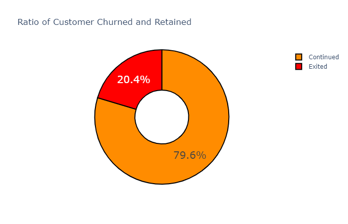
Gender
Who is loyal to the bank? Male or Female?
Gender,HasCrCard,IsActiveMember vs Churn
f,ax=plt.subplots(3,2,figsize=(18,25))
bank_data[['Gender','Exited']].groupby(['Gender']).mean().plot.bar(ax=ax[0][0])
ax[0][1].set_title('Churn vs Gender')
sns.countplot('Gender',hue='Exited',data=bank_data,ax=ax[0][1])
ax[0][1].set_title('Gender:Churned vs Retained')
bank_data[['HasCrCard','Exited']].groupby(['HasCrCard']).mean().plot.bar(ax=ax[1][0])
ax[1][0].set_title('Churn vs HasCrCard')
sns.countplot('HasCrCard',hue='Exited',data=bank_data,ax=ax[1][1])
ax[1][1].set_title('HasCrCard: Churned vs Retained')
bank_data[['IsActiveMember','Exited']].groupby(['IsActiveMember']).mean().plot.bar(ax=ax[2][0])
ax[2][0].set_title('Churn vs IsActiveMember')
sns.countplot('IsActiveMember',hue='Exited',data=bank_data,ax=ax[2][1])
ax[2][1].set_title('IsActiveMember: Churned vs Retained')
plt.show()
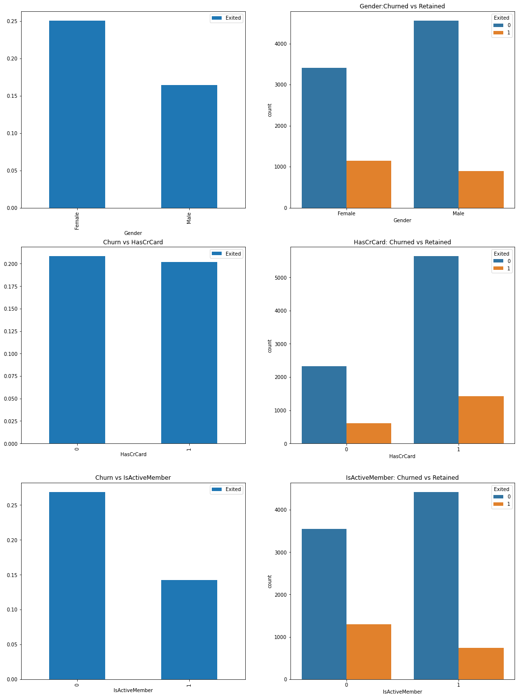
From the above graphs we can see,
-
More male customers, but when it comes to churn rate, female customers are more likely to quit the bank. (In other words, even though there are more male customers its the females who have high churn rate compared to males).
-
Majority of customers have credit cards.
-
The bank have a significant number of inactive customers. They ratio of inactive customers being churned out is high. Thus bank needs to take steps and make them active.
Geography vs Churn

The bank have majority of its customers located in France, however the chrun rate is high in Germany followed by spain, where the bank have less number of customers. This can be due to less number of branches in Germany and Spain or poor services in those regions.
Age
# peaks for Exited/not exited customers by their age
facet = sns.FacetGrid(bank_data, hue="Exited",aspect=4)
facet.map(sns.kdeplot,'Age',shade= True)
facet.set(xlim=(0, bank_data['Age'].max()))
facet.add_legend()

# average exited customers by age
fig, axis1 = plt.subplots(1,1,figsize=(18,4))
average_age = bank_data[["Age", "Exited"]].groupby(['Age'],as_index=False).mean()
average_age.columns = ['Age','Mean(Exited)']
sns.barplot(x='Age', y='Mean(Exited)', data=average_age)
del average_age


Customer having age around 48 to 60 are churning out compared to younger ones i.e., Mean(Exited) > 0.5 from the graph. The churn rate can also be due to retirement. Bank needs to revise the market strategy by focusing on keeping older customers.
bank_data[(bank_data['Age'] == 56)]['Exited'].value_counts()
1    50
0    20
Name: Exited, dtype: int64
Out of 70 people whose age equals 56, 50 of them churned out.
Tenure
y0 = bank_data.Tenure[bank_data.Exited == 0].values
y1 = bank_data.Tenure[bank_data.Exited == 1].values

fig = go.Figure()
fig.add_trace(go.Box(y=y0, name='Continued',
                marker_color = 'lightseagreen'))
fig.add_trace(go.Box(y=y1, name = 'Exited',
                marker_color = 'indianred'))

fig.update_layout(
    yaxis_title='Tenure'
)

fig.show()
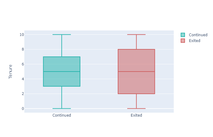
With respect to Tenure, Customers repaying loans in less years or taking more time to repay loans are churning out. Bank needs to provide benefits for customers who are repaying loans in quick time and for those who have stayed for a long time (High tenure).
Balance
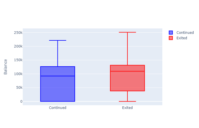
We can see that Customers having balance even after churning out.
Even though the gap is not very high yet the Customers with high account balance are churning out. This may even be due to the data imbalance. To be on the safer side the bank needs to address this as it will impact their profit.
Correlation check!
cordata = bank_data.corr(method ='pearson')
cordata.style.background_gradient(cmap='summer')
Age has some correlation (28.5%) with Churn rate. There are no real highly correlated features. NumberOfProducts and Balance are 30.4% Correlated among themselves. Apart from that there are no multi-collinear features which is good.
Let’s try and create some features [feature engineering]. Let’s See if we can create more useful features.
Feature Engineering
One of the most important part in a data science/ml pipeline is the ability to create good features. Feature Engineering is the hard skill and this is where the creativity & knowledge of data scientist/ML practioner is required.
Train, Validation and Test Split
Before we create feature we will split the data into Train, CV and Test sets. Otherwise, there will this problem of data leakage.
# train cv test split - stratified sampling
from sklearn.model_selection import train_test_split
X_train, X_test, y_train, y_test = train_test_split(X, y, test_size=0.20, stratify=y,random_state = 17)
X_train, X_cv, y_train, y_cv = train_test_split(X_train, y_train, test_size=0.20, stratify=y_train,random_state = 17)

# reset index
X_train = X_train.reset_index(drop = True)
X_cv = X_cv.reset_index(drop = True)
X_test = X_test.reset_index(drop = True)

print("train dimensions: ",X_train.shape, y_train.shape)
print("cv dimensions: ",X_cv.shape, y_cv.shape)
print("test dimensions: ",X_test.shape, y_test.shape)
train dimensions:  (6400, 10) (6400,)
cv dimensions:  (1600, 10) (1600,)
test dimensions:  (2000, 10) (2000,)
We will create features on train cv and test. Note: fit must only happen on train set.
# CreditScore and Age -- if a young man has a high credit score?
X_train['creditscore_age_ratio'] = X_train['CreditScore'] / X_train['Age']
X_cv['creditscore_age_ratio'] = X_cv['CreditScore'] / X_cv['Age']
X_test['creditscore_age_ratio'] = X_test['CreditScore'] / X_test['Age']

# log feature?
X_train['creditscore_age_ratio_log'] = np.log10(X_train['creditscore_age_ratio'])
X_cv['creditscore_age_ratio_log'] = np.log10(X_cv['creditscore_age_ratio'])
X_test['creditscore_age_ratio_log'] = np.log10(X_test['creditscore_age_ratio'])

# Given his/her age does he/she have a better credit score
mean_age = np.mean(X_train['Age']) # use mean of train data for cv and test set
mean_credit = np.mean(X_train['CreditScore']) # use mean of train data for cv and test set
.
.
.
.
# higher salary compared to his/her age?
mean_salary = np.mean(X_train['EstimatedSalary']) # mean sestimated alary of train set
X_train['high_salary_age'] = [1 if (i > mean_salary and j < mean_age) else 0 for i,j in zip(X_train['EstimatedSalary'],X_train['Age'])]
X_cv['high_salary_age'] = [1 if (i > mean_salary and j < mean_age) else 0 for i,j in zip(X_cv['EstimatedSalary'],X_cv['Age'])]
X_test['high_salary_age'] = [1 if (i > mean_salary and j < mean_age) else 0 for i,j in zip(X_test['EstimatedSalary'],X_test['Age'])]

print("New features created!")
X_train.head(3)
New features created!
| CreditScore | Geography | Gender | Age | Tenure | Balance | NumOfProducts | HasCrCard | IsActiveMember | EstimatedSalary | balance_salary_ratio | balance_or_not | creditscore_age_ratio | creditscore_age_ratio_log | Better_Age_Credit | Better_Age_Credit_Active | multi_products | Valuable_customer | tenure_age_ratio | high_salary_age | |
|---|---|---|---|---|---|---|---|---|---|---|---|---|---|---|---|---|---|---|---|---|
| 0 | 640 | Spain | Male | 43 | 9 | 172478.156250 | 1 | 1 | 0 | 191084.406250 | 0.902628 | 1 | 14.883721 | 1.172712 | 0 | 0 | 0 | 0 | 0.209302 | 0 |
| 1 | 850 | France | Female | 24 | 6 | 0.000000 | 2 | 1 | 1 | 13159.900391 | 0.000000 | 0 | 35.416667 | 1.549208 | 1 | 1 | 1 | 1 | 0.250000 | 0 |
| 2 | 494 | Germany | Female | 38 | 7 | 174937.640625 | 1 | 1 | 0 | 40084.320312 | 4.364241 | 1 | 13.000000 | 1.113943 | 0 | 0 | 0 | 0 | 0.184211 | 0 |
3 rows × 22 columns
We have created some features, but we don’t know how useful it will be. We will check their influence at the time of creating Models.
Also note that ratio features like balance_salary_ratio, creditscore_age_ratio, etc may create multi-collinearity.
Note: It has been stated that multi-collinearity is not an issue when using sckit-learn models. Source
Data Preprocessing
Preparing data for Model building.! Encoding categorical data and normalizing numerical data.
Encoding Categorical data: Gender and Geography
# Encoding Gender
X_train['Gender'] = X_train['Gender'].apply(lambda x: 1 if x == 'Male' else 0)
X_cv['Gender'] = X_cv['Gender'].apply(lambda x: 1 if x == 'Male' else 0)
X_test['Gender'] = X_test['Gender'].apply(lambda x: 1 if x == 'Male' else 0)
# One Hot Encoding - Geography
from sklearn.preprocessing import OneHotEncoder

# left-to-right column order is alphabetical (France, Germany, Spain)
ohe = OneHotEncoder(sparse=False)
X_train_geo_ohe = pd.DataFrame(ohe.fit_transform(X_train[['Geography']]),columns = ['France', 'Germany', 'Spain'])
X_cv_geo_ohe = pd.DataFrame(ohe.transform(X_cv[['Geography']]),columns = ['France', 'Germany', 'Spain'])
X_test_geo_ohe = pd.DataFrame(ohe.transform(X_test[['Geography']]),columns = ['France', 'Germany', 'Spain'])

# drop the Geography column
X_train.drop('Geography',axis=1,inplace = True)
X_cv.drop('Geography',axis=1,inplace = True)
X_test.drop('Geography',axis=1,inplace = True)

# Concat the One Hot encoded columns
X_train = pd.concat([X_train, X_train_geo_ohe],axis = 1)
X_cv = pd.concat([X_cv, X_cv_geo_ohe],axis = 1)
X_test = pd.concat([X_test, X_test_geo_ohe],axis = 1)
Data Standardization
Each feature is of different scales/units. Features like Salary and Balance have higher range of values compared to Age, Tenure. We need to standardise features before feeding them into our Models.
from sklearn.preprocessing import StandardScaler
# features to standardise
cols_norm = ['CreditScore','Age','Tenure','Balance','NumOfProducts','EstimatedSalary','balance_salary_ratio',
            'creditscore_age_ratio','creditscore_age_ratio_log','tenure_age_ratio']

sc = StandardScaler()
sc.fit(X_train[cols_norm]) # fit has to happen only on train set

X_train[cols_norm] = sc.transform(X_train[cols_norm])
X_cv[cols_norm] = sc.transform(X_cv[cols_norm])
X_test[cols_norm] = sc.transform(X_test[cols_norm])

print("Standardized!")
X_train.head()
Standardized!
Model
We will try multiple types of algorithms for this data.
- Logistic Regression
- XGBoost
- XGBoost with SMOTE Oversampling
Logistic Regression
We will use sklearn’s Logistic Regression with Hyperparameter Tuning
from sklearn.linear_model import LogisticRegression
from sklearn.metrics import roc_auc_score
from tqdm import tqdm
train_auc = []
cv_auc = []
C_list = [0.0001, 0.001 ,0.01 ,0.1, 1, 10, 100, 1000] # list of various inverse of lambda values we want to compare.
for i in tqdm(C_list): # for each values of C_list (i)
    lr = LogisticRegression(C=i,class_weight='balanced', random_state=17, solver = 'liblinear') # initialize Logistic Model with C = i
    lr.fit(X_train, y_train) # fit the lr model on the train data
    y_train_pred = batch_predict(lr, X_train) # Predict on the train data
    y_cv_pred = batch_predict(lr, X_cv) # Predict on cross validation data
    # roc_auc_score(y_true, y_score) the 2nd parameter should be probability estimates of the positive class
    # not the predicted outputs
    train_auc.append(roc_auc_score(y_train,y_train_pred))
    cv_auc.append(roc_auc_score(y_cv, y_cv_pred))

plt.plot(C_list, train_auc, label='Train AUC')
plt.plot(C_list, cv_auc, label='CV AUC')
plt.xscale('log') # change the scale of x axis
plt.autoscale(True)
plt.scatter(C_list, train_auc, label='Train AUC points')
plt.scatter(C_list, cv_auc, label='CV AUC points')
plt.xscale('log')
plt.legend()
plt.xlabel("C: hyperparameter")
plt.ylabel("AUC")
plt.title("ERROR PLOTS")
plt.grid()
plt.show()
100%|██████████| 8/8 [00:00<00:00, 16.11it/s]
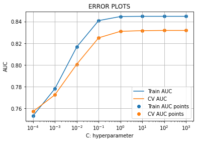
From the above image we can see that at C = 10 the train and cross validation AUC scores are high as well as close to each other. Therefore we can set the optimum C as 10.
After building the Logistic Regression model using C = 10 on train data, we get the AUC scores on train and test as shown below.
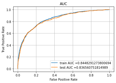
Logistic Regression - Test AUC: 0.836560751814989
Logistic Regression Feature importances
> In Logistic Regression when the absolute weights are large then w.T*x is also large.

> Weights of the feature indicate their importance.
| Weights | Abs_Weights | Features | |
|---|---|---|---|
| 15 | -5.567203 | 5.567203 | multi_products |
| 12 | -2.543284 | 2.543284 | creditscore_age_ratio_log |
| 5 | 2.352321 | 2.352321 | NumOfProducts |
| 20 | 1.474438 | 1.474438 | Germany |
| 7 | -1.005711 | 1.005711 | IsActiveMember |
| 0 | 0.949018 | 0.949018 | CreditScore |
| 11 | 0.769292 | 0.769292 | creditscore_age_ratio |
| 2 | -0.733009 | 0.733009 | Age |
| 16 | 0.698971 | 0.698971 | Valuable_customer |
| 1 | -0.605773 | 0.605773 | Gender |
| 21 | 0.581897 | 0.581897 | Spain |
| 19 | 0.533779 | 0.533779 | France |
| 18 | -0.498421 | 0.498421 | high_salary_age |
| 13 | -0.425378 | 0.425378 | Better_Age_Credit |
| 17 | 0.339650 | 0.339650 | tenure_age_ratio |
| 3 | -0.323940 | 0.323940 | Tenure |
| 8 | 0.173293 | 0.173293 | EstimatedSalary |
| 14 | -0.154712 | 0.154712 | Better_Age_Credit_Active |
| 10 | -0.092624 | 0.092624 | balance_or_not |
| 9 | 0.023764 | 0.023764 | balance_salary_ratio |
| 4 | 0.010782 | 0.010782 | Balance |
| 6 | 0.002682 | 0.002682 | HasCrCard |
From the absolute weights we can see features like ‘multi_products’,’creditscore_age_ratio_log’,’NumOfProducts’,’Germany’, ‘IsActiveMember’ are most important and features like ‘HasCrCard’,’Balance’, and ‘balance_salary_ratio’ are least important.
So feature engineering has helped alot.
Let’s drop the least important features and build the model again. From the absolute weights we can see features like ‘multi_products’,’creditscore_age_ratio_log’,’NumOfProducts’,’Germany’, ‘IsActiveMember’ are most important and features like ‘HasCrCard’,’Balance’, and ‘balance_salary_ratio’ are least important.
So feature engineering has helped alot.
Let’s drop the least important features and build the model again.
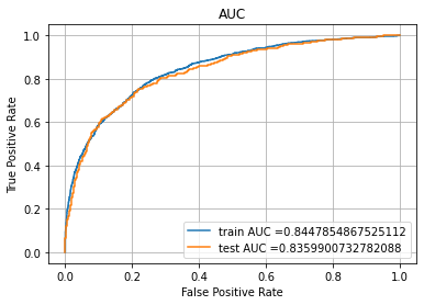
Logistic Regression - Test AUC: 0.8359900732782088
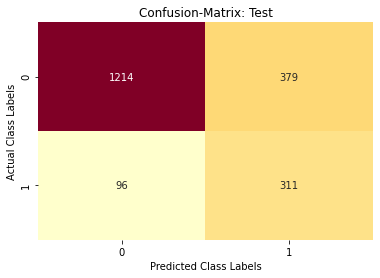
Now lets predict on test data with best threshold and see the confusion matrix.
The maximum value of tpr*(1-fpr) 0.5908667088827037 for threshold 0.488

Confusion matrix: Train data
## Classification report
from sklearn.metrics import classification_report
cr = classification_report(y_test,predict_with_best_t(y_test_pred, best_t))
print(cr)
              precision    recall  f1-score   support

           0       0.93      0.76      0.84      1593
           1       0.45      0.76      0.57       407

    accuracy                           0.76      2000
   macro avg       0.69      0.76      0.70      2000
weighted avg       0.83      0.76      0.78      2000
XGBoost Model
XGBoost documentation - Here
XGboost tutorial - Here
import xgboost as xgb

train_auc = []
cv_auc = []
n_trees = [50,100,200,300,500,750,1000] # list of various n_estimator values we want to compare.
l_rate = [0.0001,0.001,0.01,0.1,1.0,10] # list of various learning rate values we want to compare.

hyperparams = [(n,l) for n in n_trees for l in l_rate]
hyperparameter_indices = uniform_random_sample(0,len(hyperparams),size = 15)
params_list = [hyperparams[i] for i in hyperparameter_indices]
n_trees_ls = [i[0] for i in params_list]
l_rate_ls = [i[1] for i in params_list]

for i in tqdm(params_list):
    # initialize XGBoost Model with n_estimators = i[0] and learning_rate = i[1]
    xg = xgb.XGBClassifier(n_estimators=i[0],learning_rate=i[1],random_state = 17)
    xg.fit(X_train, y_train) # fit the Xgboost model on the train data
    y_train_pred = batch_predict(xg, X_train) # Predict on the train data
    y_cv_pred = batch_predict(xg, X_cv) # Predict on cross validation data
    # roc_auc_score(y_true, y_score) the 2nd parameter should be probability estimates of the positive class
    # not the predicted outputs
    train_auc.append(roc_auc_score(y_train,y_train_pred))
    cv_auc.append(roc_auc_score(y_cv, y_cv_pred))
100%|██████████| 15/15 [00:48<00:00, 3.20s/it]
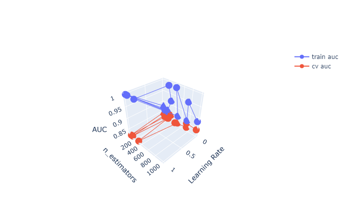
From the above plot we can see the best set of parameters are best_n_estimator = 500 & best_l_rate = 0.01
After building the XGBoost classifier using best_n_estimator = 500 & best_l_rate = 0.01, we get Train and Test AUC scores as follows:
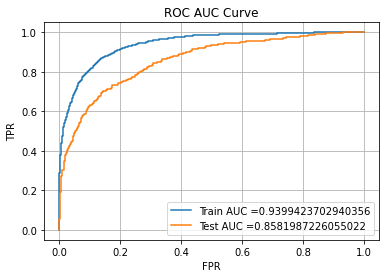
XGBoost --> Train AUC:  0.9399423702940356
XGBoost --> Test AUC:  0.8581987226055022
Confusion Matrix – XGBoost Model
The maximum value of tpr*(1-fpr) 0.7502817077751346 for threshold 0.224

Confusion matrix: Test data

## Classification report -- XGBoost Model
XGBoost Model:
               precision    recall  f1-score   support

           0       0.92      0.84      0.88      1593
           1       0.53      0.71      0.61       407

    accuracy                           0.81      2000
   macro avg       0.72      0.78      0.74      2000
weighted avg       0.84      0.81      0.82      2000
Model with oversampling – SMOTE Sampling
from imblearn.over_sampling import SMOTE # run "conda install -c conda-forge imbalanced-learn" in anaconda promt
sm  = SMOTE(random_state=17)
X_train_sm,y_train_sm = sm.fit_sample(X_train,y_train)
print(X_train_sm.shape,y_train_sm.shape)
(10192, 22) (10192,)
Repeating the same XGBoost model building process with Oversampled data, we get:
The maximum value of tpr*(1-fpr) 0.7712574380374055 for threshold 0.466

Confusion matrix: Test data
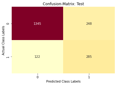
## Classification report -- XGBoost Model with SMOTE data
XGBoost Model:
                   precision    recall  f1-score   support

               0       0.92      0.84      0.88      1593
               1       0.53      0.70      0.61       407

        accuracy                           0.81      2000
       macro avg       0.73      0.77      0.74      2000
    weighted avg       0.84      0.81      0.82      2000
We can still improve the scores by adding/removing some more features or trying out other algorithms.
XGBoost Feature importance
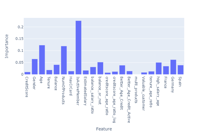
We can see that features like isActiveMember, NumofProducts & Age have major contributions towards the prediction.
Summary
+---------------------------+-----------------------------------------+--------------------+
|           Model           |             Hyper parameter             |   Auc on testset   |
+---------------------------+-----------------------------------------+--------------------+
|    Logistic Regression    |              1/λ or C = 10              | 0.8359900732782088 |
|          XGBoost          | n_estimator = 500, learning_rate = 0.01 | 0.8581987226055022 |
| XGBoost With Oversampling | n_estimator = 300, learning_rate = 0.01 | 0.8530649293361158 |
+---------------------------+-----------------------------------------+--------------------+
You can find full code here


